In the previous post I laid out an outline for the case for computerized planning. In this post I will present some simple examples that should help get the point across.
A tiny example economy
In these examples I will use an economy which produces only one good. That good could be anything, for example food. There are two technologies available to produce this good: techA and techB. The difference between the two technologies is that techA uses 2 units of labour and 3 units of CO2 emissions per unit of output while techB is the opposite: 3 units of labour and 2 units of CO2. They complement each other, and the choice between them depends on whether we're minimizing labour input, CO2 emissions or some combination of the two. Given demand , maximum labour and maximum CO2 emission , we have the following matrix equation:
Both and are non-negative, meaning . All are implied to be non-negative for the rest of this article.
On its own the preceeding equation is not very useful since neither labour nor CO2 are variables. To be able to optimize on either, the system needs to be extended. Let's start with minimizing labour, which requires adding a third variable :
The new column in the matrix turns the second row into a "balance equation". Since we are minimizing the goal is to add as little of it as possible while still keeping the sum of the labour added and the labour consumed non-negative.
The optimal solution that we seek is given by:
where
The solution depends only on and . If we let then we can sweep from 0 to 2.5. The following bash script does this, has lp_solve solve the resulting linear program, parses the result and spits out Octave code the renders the plot below:
#!/bin/bash
# makes seq use decimal dots in Swedish locale, not commas
export LANG=C

echo "x=["
for d in $(seq 0 0.05 2.5)
do
  lp_solve <<EOF > /tmp/lp_result
min: xl;
xa + xb >= $d;
-2 xa - 3 xb + xl >= 0;
-3 xa - 2 xb >= -5;
EOF
  for var in xa xb xl
  do
    V=$(grep $var /tmp/lp_result | sed -e 's/^[^0-9]*//')
    export $var=$V
  done
  echo "$d,$xa,$xb,$xl;"
done
echo "];"
echo "plot(x(:,1),x(:,2),x(:,1),x(:,3),x(:,1),x(:,4));"
echo "legend('techA','techB','labour','location','northeastoutside');"
echo "xlabel('Demand');"
echo "ylabel('Intensity');"
echo "title('CO_2 constrained labour-minimizing economy');"
echo "axis([0,2.5,0,8]);"
echo "print('tiny_economy.png');"
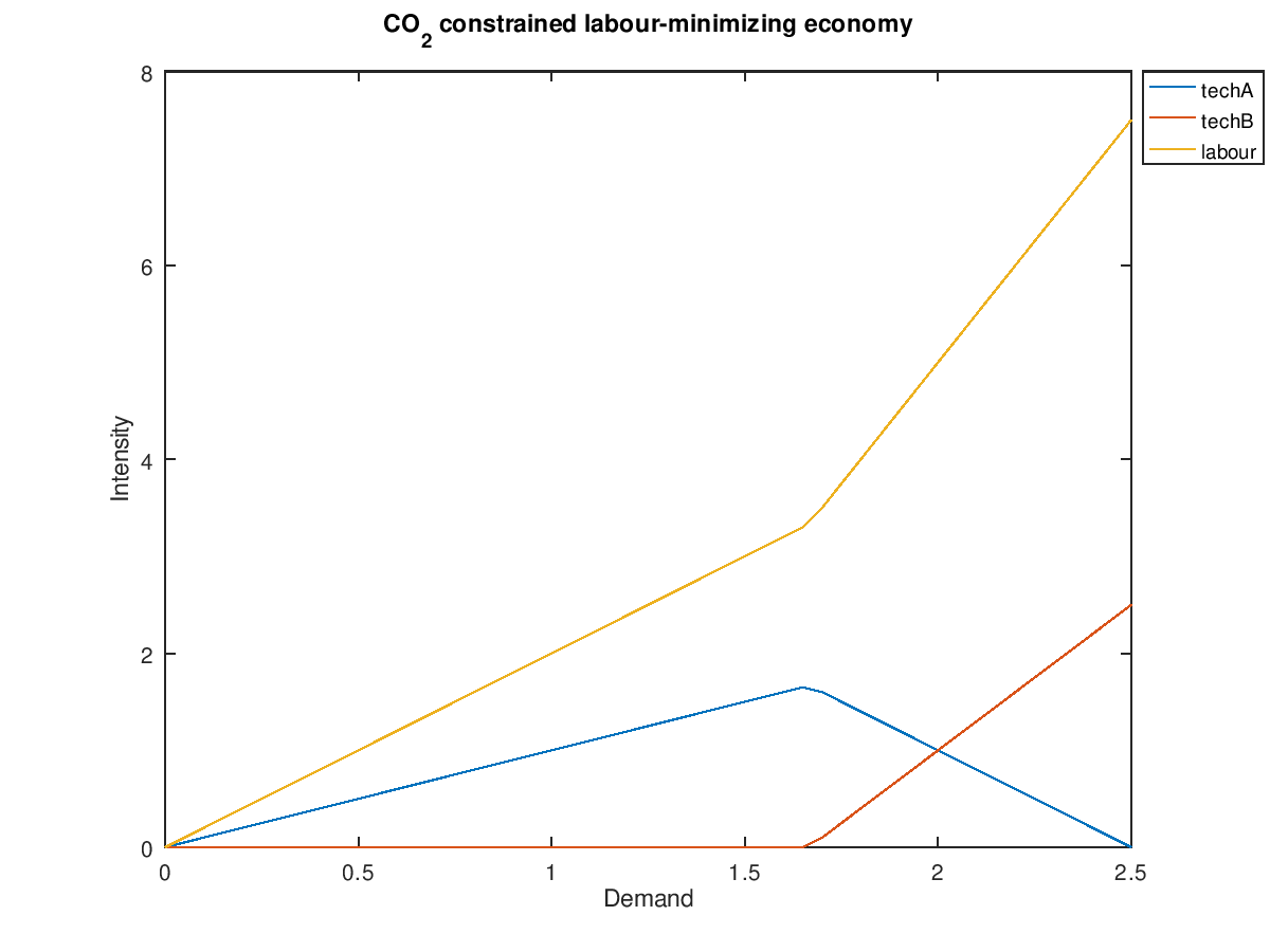
We can see that techA is preferred as long as CO2 emissions stay below the limit. Once demand goes past 1.66, techB starts getting used and the marginal demand for labour increases.
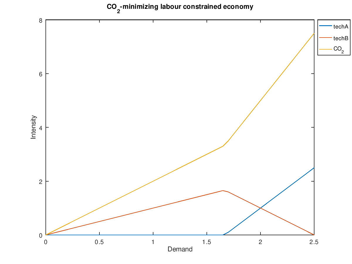
If we instead minimize CO2 emissions then the result looks much the same, except techA and techB swap roles:
#!/bin/bash
# makes seq use decimal dots in Swedish locale, not commas
export LANG=C

echo "x=["
for d in $(seq 0 0.05 2.5)
do
  lp_solve <<EOF > /tmp/lp_result
min: xc;
xa + xb >= $d;
-2 xa - 3 xb >= -5;
-3 xa - 2 xb + xc >= 0;
EOF
  for var in xa xb xc
  do
    V=$(grep $var /tmp/lp_result | sed -e 's/^[^0-9]*//')
    export $var=$V
  done
  echo "$d,$xa,$xb,$xc;"
done
echo "];"
echo "plot(x(:,1),x(:,2),x(:,1),x(:,3),x(:,1),x(:,4));"
echo "legend('techA','techB','CO_2','location','northeastoutside');"
echo "xlabel('Demand');"
echo "ylabel('Intensity');"
echo "title('CO_2-minimizing labour constrained economy');"
echo "axis([0,2.5,0,8]);"
echo "print('tiny_economy2.png');"
In reality we may want to minimize some combination of labour and CO2. The following is an interesting example:
#!/bin/bash
# makes seq use decimal dots in Swedish locale, not commas
export LANG=C

echo "x=["
for d in $(seq 0 0.05 2.5)
do
  lp_solve <<EOF > /tmp/lp_result
min: xl + 0.5 xc;
xa + xb >= $d;
-2 xa - 3 xb + xl >= 0;
-3 xa - 2 xb + xc >= 0;
xa <= 1.5;
xb <= 1.5;
xc <= 6;
EOF
  for var in xa xb xl xc
  do
    V=$(grep $var /tmp/lp_result | sed -e 's/^[^0-9]*//')
    export $var=$V
  done
  echo "$d,$xa,$xb,$xl,$xc;"
done
echo "];"
echo "plot(x(:,1),x(:,2),x(:,1),x(:,3),x(:,1),x(:,4),x(:,1),x(:,5));"
echo "legend('techA','techB','labour','CO_2','location','northeastoutside');"
echo "xlabel('Demand');"
echo "ylabel('Intensity');"
echo "title('Combination economy');"
echo "axis([0,2.5,0,8]);"
echo "print('tiny_economy3.png');"
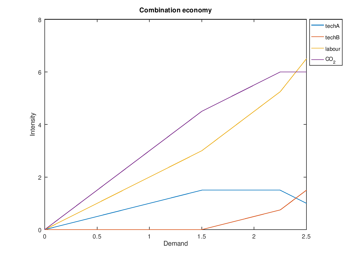
In this example the capabilities of techA and techB are limited. Each can only produce 1.5 units of goods. Additionally, CO2 emissions are limited to 6 and we're trying to optimize for a mix that favours labour. Three different regions are clearly visible. The first region is unconstrained, the second region is constrained by the capabilities of techA and the third region is constrained by CO2. As the marginal CO2 "demand"/budget decreases, the marginal demand for labour increases.
Incidentally, the equations for this system look like this:
Here I have chosen to make the non-negativity constraints on explicit, to highlight that the full matrix is tall. We can also see that the system is quite sparse and that it can be slightly simplified:
Other examples
Chain economy
A chain economy like A -> B -> C -> ... Z where each industry needs two units of the industry before it, one unit of labour and one unit of CO2, looks like this:
Service economy
Services are industries which notionally require only labour. In practice they require more than that, like office supplies. Service workers also need to eat, but that is handled elsewhere in the equations. Service industries do not emit CO2 on their own, but may do so indirectly, like all industries today.
Food production
To ensure everyone is fed and that there's a variety of foods available, one adds a number of constraints. The most important of these are those for macronutrients like energy, carbohydrates, fat, protein and so on. If we were to rely only on nutrients then the solution would likely end up picking a single crop like maize or sorghum. While this keeps people fed, it would be a very depressing diet.
We can use statistics of what kinds of food people prefer and add a constraint for each one: produce at least potatoes, coconut milk, Habaneros and so on. It is also the case that preferences vary with season and region. We know with high certainty that demand for Julmust will be high for roughly two months around the winter solstice in Sweden, but comparatively low the rest of the year. A similar peak occurs around Easter for Påskmust.
Demand for some goods vary with a frequency different from that of the Gregorian year. For example goods associated with Ramadan and similar traditions that follow a lunar calendar. For regional foods, sizeable diasporas must be accounted for.
For the ten staple foods listed on Wikipedia the following LP for how much area to plant of each crop can be built:
Each column corresponds to a staple crop from maize to plantain and the final column is for optimizing area. The values are weighted by how much is produced per hectare by the most productive country for each crop. Rows are scaled so that the values for the ninth column (sorghum) are all ones. The right-hand side is given by the RDA column in the Wikipedia article and represents how many hectares must be cultivated to produce 10,000 person-days of each nutrient.
Rows correspond to energy, protein, carbohydrates, fiber, monounsaturated fatty acids and polyunsaturated fatty acids. The final row is the balance equation for area.
We can see by visual inspection that sorghum is the most efficient crop in terms of area, with 0.26 hectares being enough to supply 10,000 person-days of macronutrients. The limiting factor is monounsaturated fatty acids. If canola oil is used for fat, then the necessary area shrinks to around 0.11 hectares.
This sort of diet would only really be acceptable in the most extreme circumstances. As I said in the beginning of this section, one would add extra constraints that certain crops should be grown because people want them. Yields also vary by location, but adding extra variables per grid locator for optimization would not fit in a blog post.