In the post Feasibility is optimal I suggested introducing a new barrier function to guarantee faster convergence towards the analytical center of a polytope. This turns out to be unnecessary or even detrimental, and in this post I will get into why. This post also presents a potentially new result relating to convergence for a class of central path methods for linear programming which I will call medium-step methods.

After digging around for literature on self-concordant functions I came across the book Convex Programming by Stephen Boyd and Lieven Vandenberghe. Chapter 9 of the book deals precisely with the kind of problem I'm wanting to solve, especially section 9.6.

I will also use the paper A polynomial-time algorithm, based on Newton's method, for linear programming by James Renegar. Using the notation from Renegar, the iteration bound on page 505 in Convex Programming, using optimal line search and 64-bit floating point accuracy, becomes:

$\frac{20-2}{1/4(1-1/2{)}^2}\left(f(\xi )-f(x_0)\right)+{\log }_2{\log }_2(1/2^{-53})\le 288\left(f(x_0)-f(\xi )\right)+6$

All that remains is to work out a bound for $\mathrm{\Delta }=f(x_0)-f(\xi )$. Remember that $f$ here is the barrier function, which we are minimizing. Large values of $\mathrm{\Delta }$ means slow convergence. In particular it is purely detrimental to add large quadratic terms as I suggested in the previous post. It may also be tempting to scale the barrier function down by some constant $r<1$ so as to reduce $\mathrm{\Delta }$ and thus the number of iterations, for example using $f(x)=r\log x$. But such scaling violates the self-concordance constraint that sits at the heart of the complexity analysis that Boyd and Vandenberghe (really Nesterov and Nemirovski) provides:

$|f^{\prime \prime \prime }(x)|\le 2f^{\prime \prime }(x{)}^{3/2}$

$2f^{\prime \prime }(x{)}^{3/2}=\frac{2r^{3/2}}{(x^2{)}^{3/2}}=\frac{2r^{3/2}}{x^3}$

$|f^{\prime \prime \prime }(x)|=\frac{2r}{x^3}$

$\frac{2r}{r{x}^3}\le \frac{2r^{3/2}}{x^3}\iff 1\le \sqrt{r}$

which is violated for $r<1$. It also makes sense that this kind of scaling should provide no benefit due to the affine invariant nature of the Newton method.

Finally, Boyd and Vandenberghe claim that Nesterov and Nemirovski provide an even tighter bound on the number of iterations, but I do not have access to the relevant work. The following PDF on Nemirovski's website may contain relevant information but I have not read it yet: Interior point polynomial time methods in convex programming

A conservative bound on Δ

To get started, let's borrow and adapt some of Renegar's notation. Renegar has the original system $Ax\ge b$ with $A\in {\mathbb{R}}^{m\times n}$. So $x$ has $n$ dimensions, and we have $m$ inequalities. Renegar also introduces $l$ extra inequalities, each one a copy of $c^{T}x\ge k^{(j)}$. These extra inequalities are moved forward at each step in the algorithm until we get close enough to the optimal solution. This is the "broom" I've written about earlier. Renegar ultimately uses $l=m$, but provides convergence analysis for other values of $l$ which shall become useful.

When modifying a constraint in a system let $m^{\prime }=m-1$ and $l=1$ where the latter corresponds to the constraint we are changing. Using $l>1$ would be useless in what follows, but I will try to preserve the analysis for other values of $l$ in case it is useful to someone.

Each step $j$ in the algorithm has an associated centroid ${\xi }^{(j)}$. Define the function ${\mathbf{\text{X}}}^{(j)}(x)$ as follows:

${\mathbf{\text{X}}}_i^{(j)}(x)=\frac{a_i^{T}x-b_i}{a_i^T{\xi }^{(j)}-b_i}$

where $1\le i\le m^{\prime }$ correspond to the constraints that are not changing and $m^{\prime }+1\le i\le m^{\prime }+l$ to the one that does change (and copies of it, if any). In other words $\mathbf{\text{X}}(x)$ normalizes the coordinates $Ax-b\in {\mathbb{R}}^m$ by dividing them elementwise by $A{\xi }^{(j)}-b$. This means that ${\mathbf{\text{X}}}^{(j)}({\xi }^{(j)})=e$ where $e$ is all ones. Renegar also shows that $e^T\mathbf{\text{X}}(x)=m=m^{\prime }+l$ for all feasible $x$.

If we move the constraint some fraction $\delta <1$ towards ${\xi }^{(j)}$, and if we started with a perfectly centered system ($\alpha ={\parallel {\mathbf{\text{X}}}^{(j)}({\xi }^{(j)})-e\parallel }_2=0$) then Renegar shows that the distance from this point to the center of the new system ($\beta ={\parallel {\mathbf{\text{X}}}^{(j+1)}({\xi }^{(j)})-e\parallel }_2$) is bounded by

${\beta }^2-\frac{l{\delta }^2}{1-\delta }\beta -\frac{l{\delta }^2}{1-\delta }\le 0$

For $l=1$ this inequality has the solution

$\beta \le \frac{\delta }{1-\delta }$

And for $l\gg 1$ and $\delta$ not too small it is roughly

$\beta \lesssim \frac{l{\delta }^2}{1-\delta }$

If for example $\delta =1/3$ and $l=1$ then $\beta =1/2$. Note that we can never perfectly center any system due to limited machine precision, so in reality $\alpha$ is somewhere around $ϵ\sqrt{m}$. This turns out to not matter in this case - this small extra contribution gets rounded off in the end.

The question now is how large can $\mathrm{\Delta }$ actually be? Let's first express it in terms of $\mathbf{\text{X}}$:

$\mathrm{\Delta }=\left[-{\sum }_i\log \left(a_i^T{\xi }^{(j)}-b_i\right)\right]-\left[-{\sum }_i\log \left(a_i^T{\xi }^{(j+1)}-b_i\right)\right]$

$=-{\sum }_i\log \left(\frac{a_i^T{\xi }^{(j)}-b_i}{a_i^T{\xi }^{(j+1)}-b_i}\right)$

$=-{\sum }_i\log \left({\mathbf{\text{X}}}_i^{(j+1)}({\xi }^{(j)})\right)$

Let's further introduce $V={\mathbf{\text{X}}}^{(j+1)}({\xi }^{(j)})-e$, meaning we have:

$\mathrm{\Delta }=-{\sum }_i\log (1+V_i)$

Note that the sum over all elements in $V$ is zero ($e^{T}V=0$). Negative elements in $V$ contribute positively to $\mathrm{\Delta }$ (meaning raising it, worsening the iteration bound) whereas positive elements contribute negatively (improving the iteration bound).

We may obtain a simple upper bound for $\mathrm{\Delta }$ by first bounding $\delta \le 1/3$ and therefore $\beta \le 1/2$. If we desire to move the constraint further than $\delta =1/3$ then we can do so in multiple steps. Next let $V$ have exactly one negative element, $-\beta$, and let's pretend that all other elements are zero. This cannot actually happen due to the zero sum constraint, so this upper bound is very conservative. We therefore have

$\mathrm{\Delta }\le -\log (1-\beta )=\log 2\approx 0.6931$

Because of the convexity and strictly decreasing nature of $-\log (1+V_i)$ there is no combination of two or more negative elements that will yield a higher upper bound on $\mathrm{\Delta }$. We therefore have

$\text{\#Iterations}\le \lceil 288\log (2)+6\rceil =206$

This is already a useful result because it means we can move any constraint a substantial portion of the distance to the current center, and recenter the system in a reasonable amount of time. In particular we do not have to perform $O(\sqrt{m})$ Newton steps as we would otherwise expect. Note that this does not help solve LP faster in general, because setting $l=1$ means overall convergence with respect to some objective function is slow. Using assumption (3.2) of Renegar with $\alpha$ explicit:

$k^{\text{opt}}-k^{(j)}\le {\left(1-(1-\alpha )\frac{\delta l}{m^{\prime }+l}\right)}^j(k^{\text{opt}}-k^{(0)})$

With $\delta =1/3$, $l=1$ and $\alpha =0$:

$k^{\text{opt}}-k^{(j)}\le {\left(1-\frac{1}{3m^{\prime }+3}\right)}^j(k^{\text{opt}}-k^{(0)})$

Which means that for every bit of desired accuracy we need to perform

$j\approx (3m^{\prime }+3)\log 2\approx 2m$

iterations, each one consisting of up to 206 Newton steps. Letting $l=m$ and $\delta =1/(13\sqrt{m})$ on the other hand results in only

$j\approx 28\sqrt{m}\log 2\approx 20\sqrt{m}$

iterations, each one only a single Newton step. We cannot use say $\delta =1/13$ with $l=m$ because then $\beta \approx m/156$ and $\mathrm{\Delta }$ will become large.

An even better bound on Δ

By making use of the sum constraint we can improve the bound on Δ.

Let $V\in {\mathbb{R}}^m$ be the vector with a single negative element, all other elements positive and equal and ${\parallel V\parallel }_2=\beta$. For convenience let

$a=\beta \frac{1}{\sqrt{m(m-1)}}$

then

$V=\left(-(m-1)a,a,\dots ,a\right)$

Clearly $e^{T}V=0$, and

${\parallel V\parallel }_2^2={\beta }^2\frac{(m-1{)}^2+m-1}{m(m-1)}={\beta }^2$

To see whether $V$ maximizes $\mathrm{\Delta }$ let us evaluate the gradient of the barrier function at $V$ projected onto the null space of $e$. First the unprojected gradient:

$g=\nabla f(V)=\left(\frac{-1}{1-(m-1)a},\frac{-1}{1+a},\dots ,\frac{-1}{1+a}\right)$

We can perform the above mentioned projection by subtracting the average of the entries in $g$ from $g$ itself:

$\hat{g}=g-e\frac{1}{m}\left(\frac{-1}{1-(m-1)a}+\frac{-(m-1)}{1+a}\right)$

$=g-e\frac{1}{m}\left(\frac{-(1+a)-(m-1)(1-(m-1)a)}{(1-(m-1)a)(1+a)}\right)$

$=g-e\frac{1}{m}\left(\frac{((m-1{)}^2-1)a-m}{(1-(m-1)a)(1+a)}\right)$

$=g-e\frac{(m-2)a-1}{(1-(m-1)a)(1+a)}$

$=\left(\frac{-1}{1-(m-1)a}-\frac{(m-2)a-1}{(1-(m-1)a)(1+a)},\frac{-1}{1+a}-\frac{(m-2)a-1}{(1-(m-1)a)(1+a)},\dots \right)$

$=\frac{1}{(1-(m-1)a)(1+a)}\left(-(1+a)-(m-2)a+1,-(1-(m-1)a)-(m-2)a+1,\dots \right)$

$=\frac{1}{(1-(m-1)a)(1+a)}\left(-(m-1)a,a,\dots ,a\right)$

In other words:

$\hat{g}=\frac{1}{(1-(m-1)a)(1+a)}V$

But because $V$ butts up against and is perpendicular to the ${\parallel V\parallel }_2=\beta$ constraint, and $\hat{g}$ points in the same direction as $V$, therefore $V$ is locally optimal. Whether it is globally optimal is something that I conjecture is true, but I cannot prove it at present. At least one other local optimum exist, $a=-\beta /\sqrt{m(m-1)}$ (signs merely flipped), but it can be shown to be inferior to its negative, as we shall soon see. Moving on, we have the following conjectural bound:

$\mathrm{\Delta }\le -\log \left(1-\beta \sqrt{\frac{m-1}{m}}\right)-(m-1)\log \left(1+\beta \sqrt{\frac{1}{m(m-1)}}\right)$

And in the limit:

${lim}_{m\to \mathrm{\infty }}\mathrm{\Delta }\le -\log (1-\beta )-\beta$

Because we have limited $\beta \le 1/2$ we therefore have

$\mathrm{\Delta }\le \log (2)-\frac{1}{2}\approx 0.1931$

If we use $a$ with signs flipped we instead get $-\log (1+\beta )+\beta \approx 0.094535$, which is inferior as previously stated. The iteration bound therefore, conjecturally, improves to:

$\text{\#Iterations}\le \lceil 288\left(\log (2)-\frac{1}{2}\right)+6\rceil =62$

We can do even better by optimizing the choice of $\delta$. The following Octave code shows that $\delta =1/6$ is optimal:

octave:58> d=0.01:0.001:0.4; b=d./(1-d); it=(ceil(288*(-log(1-b)-b))+6).*ceil(1./d/3); plot(d,it); [i,j] = min(it); it(j), d(j)
ans = 26
ans = 0.1670

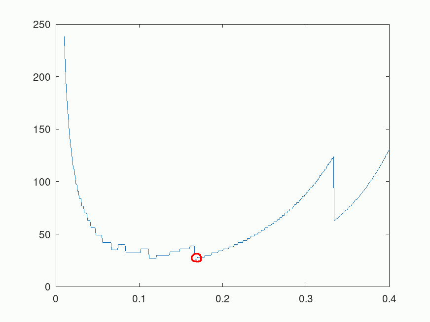
So as few as $2*13=26$ Newtons steps will perform the same job that would otherwise require 62 steps with $\delta =1/3$. So conjecturally we are nearly an order of magnitude faster than the 206 figure in the previous section.

Medium-step

The term medium-step comes about for two reasons: the existence of the term long-step in the literature and the much shorter steps taken in Renegar's paper compared to what is done here.

Renegar uses $\delta =1/(13\sqrt{m})$ whereas I use $\delta =1/6$ above. We could therefore call Renegar's $\delta$ short-step. It requires $O(L\sqrt{m})$ iterations. On the other extreme, the type of predictor-corrector methods often used in practice are known as long-step methods. They use $\delta \gg 1$, sometimes stepping as far as 99.9% of the distance to the boundary of the system. Todd and Ye demonstrate that these methods have worst-case performance of $\mathrm{\Omega }(L\sqrt[3]{m})$ and, if I understand correctly, they remain $O(L\sqrt{m})$.

Because the $\delta$ chosen above is inbetween these two extremes I have chosen to call the method medium-step. Note again that this result is only useful if we seek to remain in the center of a linear program. It is not useful if one seeks to optimize some objective function $c^{T}x$.

Future work

Further theoretical improvements could be made by analyzing what I will call medium-step predictor-corrector methods. By computing the tangent to the central path using a short step, a line search can be performed for finding a better initial guess in the system updated with $\delta =1/6$. This is likely to bring down the number of Newton steps. By how much I am not sure. Note that computing this tangent itself costs a small number of Newton steps. On the other hand the system is likely to be better conditioned compared to just after a medium-step update, meaning these Newton steps are cheaper to compute.

Closing remarks

I started writing this post around 2023-03-05, so in total I've been obsessing about this specific problem for roughly seven weeks. Initially I thought I had a much stronger result than I actually do, so quite a bit of time was spent making sure I don't overstate the result. In the process I've learned even more about barrier methods and self-concordant functions.